An Introduction to Geometric Deep Learning

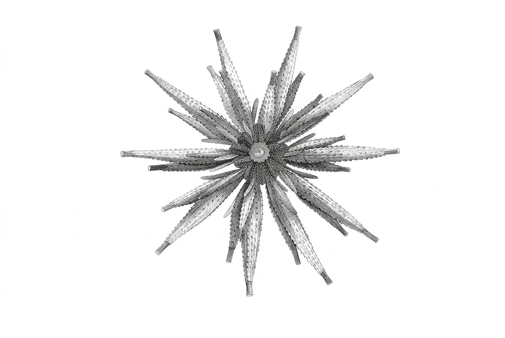
Cover image: Oken, Echinoderms and Crinoids, 1836. The echinoderm is featured by its symmetry.

Motivation

Most of the time we consider deep learning as an empirical subject. We are told what works, what doesn't, and what the standard solution is to some specific problems, yet few people have asked for the reason behind them.

This article aims to serves as a brief introduction to Geometric Deep Learning (GDL), which introduce a different way of understanding the famous Deep Learning architectures such as CNN, GCN and Transformers, explaining why these architecture designs may take the advantages of exploiting the underlying data's geometric properties.

With no need of bordering with the obscure mathematics in the original Geometric Deep Learning book, this blog wishes to give you a clean big picture by deriving the key components of CNN, DeepSets, GCN and Transformer and revealing their relations.

Before you start

No worries if you don't understand some terms in the above introduction. I've tried to explain them all from first principles as much as possible, but for a smooth reading experience, you at least ought to be familiar with the following.

• First-year level linear algebra.
• Basic knowledge about Convolutional Neural Network and Self-attention.

Here are some nice YouTube videos that give a sense of them.

• Essence of linear algebra by 3Blue1Brown
• But what is a neural network? by 3Blue1Brown
• But what is a convolution? by 3Blue1Brown

As a complement, there are some awesome materials of introductory Group Theory. To read this article, they are not a must, but they definitely help if you want to dive deeper into the formal language of GDL.

• Group Theory Step-by-Step: 1 - 7 by TheGrayCuber
• What is Group Theory? — Group Theory Ep. 1 by Nemean

Geometric Equivariance

We've talked about take the advantages of the geometric properties of the data's geometric properties. To make our language clearer, we are specifically referring the ones called the equivariance under certain transformation. The following example shows a simple model $f$ which estimates the prices of items on your desk.

Note that the input data comes as a sequence. The model should, as we expected, assign the same value to each corresponding item if we permute the order of them, despite the fact that the prices might be interdependent as a one is likely richer if they owns a more expensive Laptop.

We can conclude that such a model satisfies the equivariance under permutation. Generally speaking, that is for any input $\mathbf{x}$ after some transformation $g$, the model outputs the exact same results as if we had applied the same transformation to the output instead:

In other words, we say that the model $f$ and the transformation $g$ commute, and this is exactly what we mean by equivariance.

Assumptions like this are called inductive biases. An inductive bias is a prior belief, built into a learning algorithm before any data is seen, about which functions are likely to solve the task. A model that is equivariant by construction does not need to learn the symmetry from examples. Instead, the symmetry is already in its architecture, which usually means fewer parameters and better sample efficiency.

Many real tasks have such symmetries. A classical Computer Vision task is to categorise image data with a wide range of tags, and it is more than reasonable to design the model architecture around the equivariance of interest. In the next section we will take the simplest case, shift equivariance, and derive the core component of the Convolutional Neural Network (CNN).

Convolutional Neural Networks

To keep things simple, we will represent an image as a column vector, i.e. a single row of pixels. A barcode is a good example. It is essentially a 1D image, a row of black and white bars, where each bar plays the role of one pixel and its value records the brightness the pixel has.

With the signal written as a column vector, we can now ask what the first layer should compute. You already know that a CNN is built from convolution layers. The question here is why convolution is the natural choice among all linear layers. To answer it, look at the first layer. Whatever we do with the signal later, this layer has to turn it into a feature map. Suppose the layer acts on the signal by left multiplication with a matrix $W$, so $\mathbf{y} = W\mathbf{x}$, with $\mathbf{y}$ of the same spatial size as $\mathbf{x}$. For now we assume a single channel and no bias. Images have no preferred origin. If a pattern appears at a different position, the layer should produce the same response, shifted along with the pattern.

To make this precise, assume the signal is periodic, so positions wrap around in a circle. This is the periodic boundary condition. For example, the unit shift acts on the vector as:

Equivalently, $S$ is the permutation matrix

Aside

If you are familiar with group theory, the shifts of a periodic signal form a cyclic group:

$$G = \{S^0, S^1, \dots, S^{n-1}\}, \quad S^0 = I.$$

A few basic facts are enough.

• A shift can be composed with itself. For example, $S^2$ means applying the unit shift twice, which is the same as shifting by two pixels at once.
• Shifts can also be composed with each other, and the result is still a shift, $S^a S^b = S^{a+b}$ with the exponent taken modulo $n$. This also means every shift has an inverse; for example, $S^{n-1}$ undoes $S$.

Since every other shift is a composition of $S$ with itself, it is enough to require that $W$ commute with $S$:

This is shift equivariance. Since this holds for all $\mathbf{x}$, it becomes $W S = S W$. Pointwise nonlinearities commute with shifts, so this property survives the rest of the feature extractor. We will see that this single equation forces $W$ to be a convolution and cuts its free parameters from quadratic to linear.

Shift equivariance implies $W S = S W$, which ensures $W$ to be a circulant matrix for some parameters $\theta_0,\dots,\theta_{n-1}$ of the form:

by Theorem 1.

The subscript of $\theta$ is the cyclic offset from the diagonal, so $\theta_0$ is the diagonal entry, $\theta_1$ the first subdiagonal, and $\theta_{n-1}$ the first superdiagonal. Observe that the layer computes exactly a discrete convolution:

The vector

is the convolution kernel. That way, we naturally deduces the convolution formula from linearity and shift equivariance. Note that our kernel size is equal to the width of the image, which reduces to a smaller one as most CNN has if we manually set further weights to zero.

Theorem 1

Statement. Let $n \in \mathbb{N}$ and let $S \in \mathbb{R}^{n \times n}$ be the permutation matrix of the unit shift on a periodic grid of $n$ pixels, that is, $(S\mathbf{x})_i = x_{i-1}$ for $i = 1,\dots,n$, with indices read modulo $n$ in $\{1,\dots,n\}$. Let $W \in \mathbb{R}^{n \times n}$. If $W S = S W$, then there exist $\theta_0,\dots,\theta_{n-1} \in \mathbb{R}$ such that

$$W_{i,j} = \theta_{i-j} \quad \text{for all } i,j \in \{1,\dots,n\}.$$

The subscript of $\theta$ is also read modulo $n$, so it always lies in $\{0,\dots,n-1\}$.

Equivalently,

$$W = \begin{bmatrix} \theta_0 & \theta_{n-1} & \theta_{n-2} & \dots & \theta_1 \\ \theta_1 & \theta_0 & \theta_{n-1} & \dots & \theta_2 \\ \theta_2 & \theta_1 & \theta_0 & \dots & \theta_3 \\ \vdots & \vdots & \vdots & \ddots & \vdots \\ \theta_{n-1} & \theta_{n-2} & \theta_{n-3} & \dots & \theta_0 \end{bmatrix}.$$

Proof. The unit shift is the permutation matrix

$$S = \begin{bmatrix} 0 & 0 & \dots & 0 & 1 \\ 1 & 0 & \dots & 0 & 0 \\ 0 & 1 & \dots & 0 & 0 \\ \vdots & \vdots & \ddots & \vdots & \vdots \\ 0 & 0 & \dots & 1 & 0 \end{bmatrix}.$$

By the definition of $S$, right multiplication by $S$ shifts column $j+1$ of $W$ to column $j$, so

$$(W S)_{i,j} = W_{i,j+1}.$$

Similarly, left multiplication by $S$ shifts row $i-1$ of $W$ to row $i$, so

$$(S W)_{i,j} = W_{i-1,j}.$$

Since $W S = S W$, we obtain

$$W_{i,j+1} = W_{i-1,j} \quad \forall i,j.$$

Letting $i' = i-1$ gives

$$W_{i'+1,j+1} = W_{i',j} \quad \forall i',j.$$

Thus $W_{i,j}$ is constant along each cyclic diagonal and depends only on the cyclic offset $i-j$. Define $\theta_k := W_{k+1,1}$ for $k = 0,\dots,n-1$. Then

$$W_{i,j} = \theta_{i-j}.\;\square$$

To wrap up, shift equivariance forces the linear layer to be a convolution. That said, a practical CNN also has element-wise nonlinearities, pooling, and other details. The key here is that the GDL never specifies a complete, ready-to-use architecture. It identifies the core components that a symmetry forces. The mathematical results inform how those components should be designed, and the remaining details are engineering choices compatible with that symmetry.

In the following chapters we will meet architectures you may not be familiar with. You do not need much prior expertise in them. The GDL informs the symmetry principle that comes before the architectural details, and that principle is enough to see why each architecture is built the way it is.

DeepSets

From now on, we will focus on architectures that concern the so-called permutation equivariance. As discussed in the introduction, many kinds of data come as a set. A point cloud is a set of 3D points, and a bag of images is a set of instances. The order of the elements carries no meaning, so permuting the input should only permute the output, and a set-level prediction should not change at all.

Since the publication of Deep Sets (Zaheer et al., 2017), its simple architecture has become a standard baseline for tasks such as population statistic estimation, point cloud classification, set expansion, and outlier detection. We will derive the layer from permutation equivariance. The input is a matrix

where each row $\mathbf{x}_i \in \mathbb{R}^{1 \times d}$ is one set element, $n$ is the number of elements, and the $d$ columns are the channels. Let $P \in \mathbb{R}^{n \times n}$ be a permutation matrix, so $PX$ permutes the rows of $X$. Assume the layer is a fixed linear map $X \mapsto WX$ with $W \in \mathbb{R}^{n \times n}$. Permutation equivariance requires

Since this holds for all $X$,

By Theorem 2, since $W$ commutes with every permutation matrix, its diagonal entries are all equal and its off-diagonal entries are all equal. That is,

Equivalently,

The layer therefore computes

It is worth pausing on what this layer does. The term $\alpha \mathbf{x}_i$ keeps the element itself, and the term $\beta \sum_{j=1}^{n} \mathbf{x}_j$ merges all elements with equal weight. This makes sense for a set. With no additional structure, the only information attached to an element is its own feature vector, so every other element enters with the same weight.

Theorem 2

Statement. Let $W \in \mathbb{R}^{n \times n}$. If $W P = P W$ for every permutation matrix $P \in \mathbb{R}^{n \times n}$, then there exist $\alpha,\beta \in \mathbb{R}$ such that

$$W = \alpha I + \beta \mathbf{1}\mathbf{1}^\top.$$

Proof. For $n\le 2$ the claim follows from the first two equalities below, so assume $n\ge 3$. Let $P$ be the permutation matrix that swaps $i$ and $j$.

Right multiplication by $P$ swaps columns $i$ and $j$ of $W$, and left multiplication by $P$ swaps rows $i$ and $j$. Since $WP=PW$, the two matrices agree entry by entry.

At $(i,i)$, the entry of $WP$ is $W_{i,j}$, while the entry of $PW$ is $W_{j,i}$. Hence

$$W_{i,j}=W_{j,i}.$$

At $(i,j)$, the entry of $WP$ is $W_{i,i}$, while the entry of $PW$ is $W_{j,j}$. Hence

$$W_{i,i}=W_{j,j}.$$

For $k\notin\{i,j\}$, the $(i,k)$ entry of $WP$ is $W_{i,k}$, while the $(i,k)$ entry of $PW$ is $W_{j,k}$. Hence

$$W_{i,k}=W_{j,k}.$$

The second equality makes all diagonal entries equal and the third makes all off-diagonal entries in a fixed column equal.

For distinct $k,l$ and $m\notin\{k,l\}$, the same column-swap argument with the transposition swapping $k$ and $l$ gives $W_{m,k}=W_{m,l}$, so different columns share the same off-diagonal value.

Hence all diagonal entries equal some $d$ and all off-diagonal entries equal some $\beta$. Therefore $W=(d-\beta)I+\beta\mathbf{1}\mathbf{1}^\top$, and setting $\alpha=d-\beta$ proves the statement. $\square$

The linear layer $W$ can be read as a message aggregation matrix. Row $i$ specifies how element $i$ merges information from all elements, and $W_{ij}$ is the weight it gives to element $j$. For $W=\alpha I+\beta\mathbf{1}\mathbf{1}^\top$, every off-diagonal weight is the same $\beta$, so the aggregation cannot distinguish one neighbour from another. The matrix is fixed, so the model can only tell an element apart from the rest of the set.

Graph Convolutional Networks

A set has no structure beyond its elements. The only relation available is whether two elements are the same, which is why DeepSets can only distinguish $i=j$ from $i\ne j$. Many data sources carry richer relations, such as citations between papers, friendships between users, or bonds between atoms.

A graph is given by an adjacency matrix $A$, with $A_{ij}=1$ when nodes $i$ and $j$ are connected, and $A_{ij}=0$ otherwise. Since we now consider graph-structured data, we will refer to elements as nodes from now on.

A richer layer should let each row compute its own weights from the others, according to the graph structure. Specifically, row $\mathbf{x}_{i}$ can read any other row $\mathbf{x}_{j}$ and assign it a weight that reflects whether they are connected, written $a_{ij}$. The same node can then aggregate its neighbours differently under different graphs. This is why $W$ becomes a function of $A$. Later, we replace $W$ by a matrix $G(A) \in \mathbb{R}^{n \times n}$, a function of the adjacency matrix. The simplest choice is $G(A)=A$.

Additionally, we can map each element to a feature with a shared linear transform $W_V$ before aggregation:

Then

Because the same $W_V$ is applied to every row, $V(PX)=P\,V(X)$. The linear map therefore preserves equivariance, while giving the layer more expressive ability. The simplest choice is $W_V=I$, which gives $V(X)=X$.

To see whether $G(A)V(X)$ still holds permutation equivariance. Permuting the nodes turns the adjacency matrix into

To see why, let's write the adjacency matrix with its row and column indices,

The entry $a_{ij}$ records the edge between node $i$ and node $j$. When the nodes are relabelled by $P$, the row index and the column index has both changed. Left multiplication by $P$ permutes the rows, and right multiplication by $P^\top$ permutes the columns, hence the permuted matrix is $PAP^\top$.

Theorem 3 shows that replacing the fixed layer $WX$ by $G(A)V(X)$, which depends on the graph, keeps the layer permutation equivariant as long as $G$ satisfies

Theorem 3

Statement. Let $G: \mathbb{R}^{n \times n} \to \mathbb{R}^{n \times n}$ and $V: \mathbb{R}^{n \times d} \to \mathbb{R}^{n \times d'}$. Define $Y(X,A)=G(A)V(X)$. If

$$G(PAP^\top) = P\,G(A)\,P^\top, \qquad V(PX) = P\,V(X)$$

for every permutation matrix $P \in \mathbb{R}^{n \times n}$, then $Y$ is permutation equivariant,

$$Y(PX,PAP^\top) = P\,Y(X,A)$$

for every $P$, $X$, and $A$.

Proof. For any permutation matrix $P$,

$$\begin{aligned} Y(PX,PAP^\top) &= G(PAP^\top)V(PX) \\ &= P\,G(A)\,P^\top P\,V(X) \\ &= P\,G(A)V(X) \\ &= P\,Y(X,A), \end{aligned}$$

where $P^\top P = I$. $\square$

For Graph Convolutional Networks (GCN), $G(A)$ is the symmetric normalised propagation matrix. Add edge on each node to itself so that each node keeps its own features:

where $\delta_{ij}=1$ when $i=j$ and $0$ otherwise. The degree of node $i$ in $\tilde A$ is

and the degree matrix is

The symmetric normalized propagation matrix is

In the framework $Y=G(A)V(X)$, the GCN layer applies a pointwise nonlinearity:

where $V(X)=XW_V$ and $W_V \in \mathbb{R}^{d \times d'}$ is the learnable linear transform.

Under a permutation $P$, the features and the adjacency matrix transform together:

Then

so

Also $V(X')=P\,V(X)$. By Theorem 3,

Self-Attention

Since the publication of Attention is all you need (Vaswani et al., 2017), this very mechanism has been applied across a wide range of tasks, such as natural language processing (NLP), audio processing and computer vision.

In this chapter, we will discuss how to design a layer enables row compute its own weights from the others, according to their content. Specifically, row $\mathbf{x}_{i}$ can read any other row $\mathbf{x}_{j}$ and assign it a weight that reflects its relevance to $\mathbf{x}_{i}$, written $g(\mathbf{x}_{i},\mathbf{x}_{j})$. The same element can then aggregate the set differently under different inputs. This is why $W$ becomes a function of $X$. Later, we replace $W$ by a matrix $G(X) \in \mathbb{R}^{n \times n}$ measuring relevance between rows.

Each element is projected into a query, a key, and a value:

with $W_Q, W_K \in \mathbb{R}^{d \times d_k}$ and $W_V \in \mathbb{R}^{d \times d'}$.

The relevance of element $j$ to element $i$ is the scaled dot product of its query and key:

A row-wise softmax turns these scores into aggregation weights:

The layer output is

Theorem 4

Statement. Let $G: \mathbb{R}^{n \times d} \to \mathbb{R}^{n \times n}$ and $V: \mathbb{R}^{n \times d} \to \mathbb{R}^{n \times d'}$. Define $Y(X)=G(X)V(X)$. If

$$G(PX) = P\,G(X)\,P^\top, \qquad V(PX) = P\,V(X)$$

for every permutation matrix $P \in \mathbb{R}^{n \times n}$, then $Y$ is permutation equivariant,

$$Y(PX) = P\,Y(X)$$

for every $P$ and $X$.

Proof. For any permutation matrix $P$,

$$\begin{aligned} Y(PX) &= G(PX)V(PX) \\ &= P\,G(X)\,P^\top P\,V(X) \\ &= P\,G(X)V(X) \\ &= P\,Y(X), \end{aligned}$$

where $P^\top P = I$. $\square$

Self-attention satisfies both conditions. Substitute $PX$ into the projections:

so the score matrix becomes

The row-wise softmax commutes with the simultaneous row and column permutation, hence

Also $V(PX) = (PX)W_V = P\,V(X)$. Theorem 4 then gives

Softmax is a design choice. Equivariance only requires $G(PX)=P\,G(X)\,P^\top$; any weight function with this property works. Softmax makes the weights nonnegative and row-normalized, which is convenient for training.

Self-attention is the case $G=G(X)$. GCN is the case $G=G(A)$, and DeepSets is the case where $G$ is constant. All three fit the same framework

Putting it all together

In the unified form

the architectures discussed so far differ in the aggregation matrix $G$ and in the symmetry they respect.

CNN uses a fixed circulant aggregation:

which commutes with the cyclic shift. Its symmetry group is the cyclic group of shifts, while the other three use the full permutation group.

DeepSets uses a fixed aggregation:

GCN uses the symmetric normalized adjacency:

Self-attention computes the weights from the content:

So CNN depends on the cyclic offset, DeepSets depends only on identity, GCN depends on graph structure, and self-attention depends on content.

Aside

The name of GCN deserves a final comment. Every shift is a permutation, so a CNN is a special case of a GCN on a fixed regular graph. Each pixel is a node, and the pixels covered by the kernel are its neighbours. The adjacency matrix of this graph is circulant, so the aggregation matrix is a convolution matrix. GCN extends this aggregation to an arbitrary graph, which is why the name keeps the word convolutional.

References

• Bronstein, M. M., Bruna, J., Cohen, T., & Veličković, P. (2021). Geometric deep learning: Grids, groups, graphs, geodesics, and gauges. arXiv preprint arXiv:2104.13478.
• Kipf, T. N., & Welling, M. (2017). Semi-supervised classification with graph convolutional networks. In Proceedings of the 5th International Conference on Learning Representations (ICLR).
• LeCun, Y., Bottou, L., Bengio, Y., & Haffner, P. (1998). Gradient-based learning applied to document recognition. Proceedings of the IEEE, 86(11), 2278–2324.
• Vaswani, A., Shazeer, N., Parmar, N., Uszkoreit, J., Jones, L., Gomez, A. N., Kaiser, Ł., & Polosukhin, I. (2017). Attention is all you need. In Advances in Neural Information Processing Systems (Vol. 30, pp. 5998–6008).
• Zaheer, M., Kottur, S., Ravanbakhsh, S., Póczos, B., Salakhutdinov, R., & Smola, A. J. (2017). Deep sets. In Advances in Neural Information Processing Systems (Vol. 30, pp. 3391–3401).