Universal Approximation Theorem

Introduction

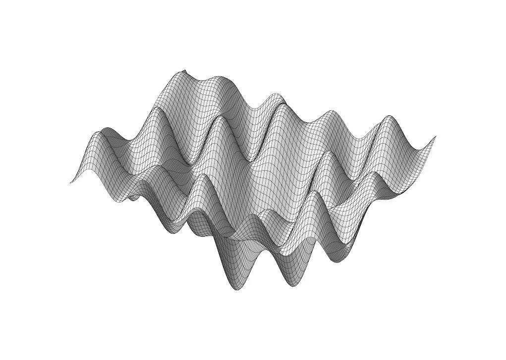
One of the most important theoretical results in neural networks is the Universal Approximation Theorem (UAT). It answers a very basic question. Can a neural network approximate any continuous function? Cybenko's 1989 result says yes. A sufficiently wide single-hidden-layer neural network can approximate any continuous function arbitrarily well.

This conclusion is easy to misread. It is an existence result. It does not guarantee that a training algorithm will find the required weights. It focuses on representational capacity. Efficiency, optimisation, and generalisation are separate questions. This naturally raises another question. If one hidden layer is already enough, why do modern models stack dozens or even hundreds of layers?

This article first states the theorem precisely, then follows Nielsen's constructive proof. We build a step function from sigmoid neurons, construct a bump from two step functions, and approximate a continuous function with a Riemann sum. After that, we discuss depth separation, the hierarchical representation hypothesis, scaling laws, and hierarchical composition in natural language. The goal is to answer a simple question. If one layer is enough, why go deeper?

Question

Machine learning is often described as function approximation. Given an input $x$ , a model produces an output $y$ . Training tries to find a function $f$ such that $f(x)$ is close to the true label. Image classification works this way. Language modelling works this way too. A network can map a picture of a planarian to the label “planarian”, and it can map a piece of text to a probability distribution over the next token.

A natural question follows. How rich is the class of functions that a neural network can represent? If it can represent only a narrow family of functions, many tasks would be impossible in principle. The Universal Approximation Theorem gives a very strong answer.

Universal Approximation Theorem

Let $S\subset\mathbb{R}^n$ be a compact set, and let $f:S\to\mathbb{R}$ be continuous. For every $\varepsilon>0$ , there exists a single-layer neural network

G(x)=\sum_{i=1}^{N}a_i\sigma(w_i\cdot x+b_i)

such that

|G(x)-f(x)|<\varepsilon,\qquad \forall x\in S.

Here $\sigma$ is the sigmoid activation function, $w_i$ are the input-to-hidden weights, $b_i$ are the biases, $a_i$ are the hidden-to-output weights, and $N$ is the number of hidden neurons.

The four key words in the theorem are continuous, single hidden layer, sigmoid activation, and arbitrary precision.

Arbitrary precision does not mean exact equality. It means that for any prescribed error tolerance $\varepsilon$ , we can find a set of parameters whose error is smaller than $\varepsilon$ . We may choose $\varepsilon=0.1$ , $0.01$ , or $0.001$ . The network usually has to grow as the tolerance becomes tighter.

The theorem also says nothing about how large $N$ must be. The constructive proof may require a very large $N$ . In practice, we care about how many neurons, layers, and data points are needed to learn the function. That is the question we turn to later.

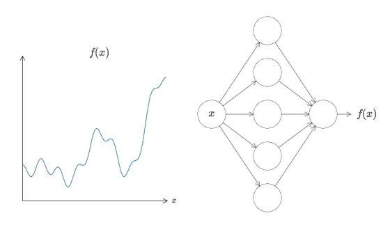
Figure 1. An arbitrary continuous function (left) and a single-hidden-layer network (right). The network approximates the target by summing a collection of sigmoid responses from the hidden layer.

The UAT is an existence theorem. It guarantees that some set of weights exists. It does not guarantee that gradient descent will find those weights from a random initialisation, and it does not guarantee that the network will generalise to new samples. Those are questions about optimisation and statistical learning, and the UAT does not answer them.

Proof

To understand why a single hidden layer has this power, we can follow the visual constructive proof of Michael Nielsen (2015). The goal is to build increasingly complicated functions from neurons, while leaving the full mathematical details aside.

The construction has four steps. We build a step function from a sigmoid, construct a bump from two step functions, approximate a continuous function with many bumps, and then extend the construction from one dimension to higher dimensions.

Step Functions

A single neuron computes $\sigma(w\cdot x+b)$ . The sigmoid is defined as

\sigma(z)=\frac{1}{1+e^{-z}}.

When $w$ is large, the sigmoid rises from 0 to 1 very quickly near $w\cdot x+b=0$ . Let the threshold be

s=-\frac{b}{w}.

Then

\sigma(wx+b)\approx \begin{cases} 1, & x>s,\\ 0, & x\le s. \end{cases}

A larger $w$ makes the transition sharper, and $b$ controls the position of the threshold. A single neuron can therefore approximate a step function.

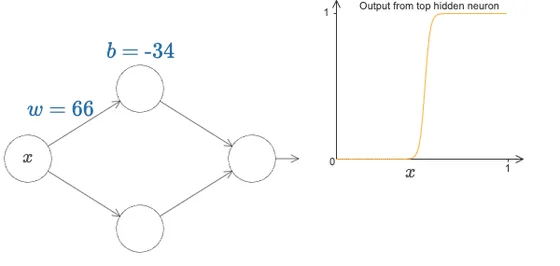
Figure 2 shows a concrete example. The hidden neuron has weight $w=66$ and bias $b=-34$ , so the threshold is $s=34/66\approx0.515$ . The output is almost a step function that jumps at $s$ .

Figure 2. A sigmoid neuron approximates a step function when the weight is large. In this example, $w=66$ and $b=-34$.

Constructing a Bump

A step function has only one jump. Subtracting two step functions that face in opposite directions produces a rectangle of finite width.

h\big(\sigma(wx+b_1)-\sigma(wx+b_2)\big) \approx \begin{cases} h, & s_1<x<s_2,\\ 0, & \text{otherwise}. \end{cases}

Here $s_1=-b_1/w$ and $s_2=-b_2/w$ , and $h$ is the height of the bump.

The network in Figure 3 has two hidden neurons with thresholds $s_1=0.40$ and $s_2=0.60$ . Their output weights are $a_1=0.8$ and $a_2=-0.8$ . Subtracting the two step functions produces a rectangular bump of height 0.8 and width 0.2.

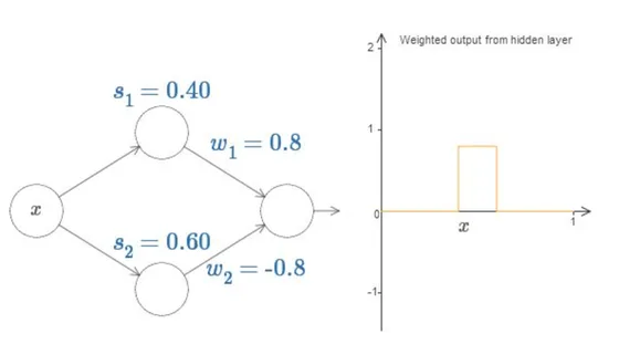
Figure 3. A bump constructed by subtracting two step functions. Changing $s_1$ and $s_2$ moves the bump and changes its width, while changing $h$ changes its height.

This step is the core of the construction. One neuron provides one boundary. Two neurons can enclose an interval. Placing many such bumps side by side covers the whole domain.

Approximating Continuous Functions

Given a continuous function $f(x)$ , divide the interval into many small pieces. On each piece, replace the function with a bump whose height is close to $f(x_i)$ . Adding all the bumps gives

G(x)=\sum_{i=1}^{M}h_iB_i(x),

where $B_i(x)$ is the $i$ -th bump and $h_i$ is its height. As the pieces become narrower and the number of bumps grows, the sum approaches the Riemann sum of $f(x)$ , and the error can be made smaller than any prescribed $\varepsilon$ .

Figure 4 shows the one-dimensional idea. The height of each orange bar is controlled by the output weight, and the width of the bar is controlled by two thresholds. If the bars are fine enough, the step curve stays close to the target function.

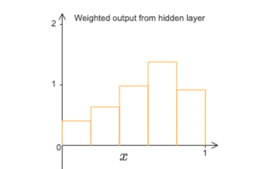
Figure 4. Approximating a continuous function with many local bumps. Each bar corresponds to a group of hidden neurons, and the output weight sets its height.

In terms of network structure, each bump needs two hidden neurons, so $M$ bumps require roughly $2M$ hidden neurons. The theorem guarantees that a sufficiently large $N$ exists. It does not say that $N$ is small. This is an important limitation of the UAT in practice.

To Higher Dimensions

An interval in one dimension becomes a region in two dimensions and a small cell in $n$ dimensions. A single sigmoid neuron still approximates the indicator of a half-space. Subtracting two half-spaces produces a strip, and combining several half-spaces can enclose smaller cells. Adding the bumps on each cell gives a piecewise approximation of a multidimensional function.

Figure 5 shows the two-dimensional construction. The inputs $x$ and $y$ pass through two groups of hidden neurons, each responsible for a step in one direction. The output layer combines the two responses into a two-dimensional bump. The panels on the right show two such bumps and the surface formed by summing many bumps.

Figure 5. The construction for two-dimensional inputs. The network on the left produces step responses for each input dimension; the panels on the right show two bumps and the surface formed by summing many bumps.

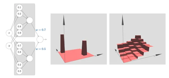
The details of the higher-dimensional proof are more involved, but the idea is the same as in one dimension. Neurons create local responses, and the local responses are added together. This completes the constructive proof.

Why Deep Learning?

The UAT answers the question “can it be represented?” It does not answer three other questions. How many neurons are needed, can the network be trained, and can it generalise?

Modern networks often have dozens or hundreds of layers. Deep networks also bring new difficulties, including vanishing gradients, exploding gradients, and highly non-convex optimisation. If one layer is already enough, why accept these difficulties?

One key difference is representational capacity versus representational efficiency. A shallow network can represent the same function, but it may need exponentially more neurons. A deep network can represent it with far fewer parameters. Depth separation is the theoretical tool that describes this difference.

Another difference comes from the hierarchical structure of data. Images, language, and sound all contain hierarchical compositions from local features to whole objects. The structure of a deep network matches this hierarchy, which can make learning easier.

Depth Separation

Depth separation concerns a class of functions with a hierarchical composition structure. A shallow network needs exponentially many neurons to represent them, while a deep network needs only linearly or polynomially many.

In formula form, there exist function families for which

N_{\text{shallow}}=\Omega(2^k), \qquad N_{\text{deep}}=O(k),

where $k$ is the number of composition layers. A shallow network can still represent these functions. It simply needs a very large width.

A classic example is the repeated composition of a triangle wave. Define

\Delta(x)= \begin{cases} 2x, & 0\le x\le \frac12,\\ 2-2x, & \frac12<x\le 1, \end{cases}

and let

f(x)=\Delta^{(k)}(x),

which is $\Delta$ composed with itself $k$ times. Each composition doubles the number of oscillations. After $k$ compositions, the function has $2^k$ linear pieces. A shallow network would need exponentially many neurons to place all these turns in one layer. A deep network can let each layer perform one composition, so it needs only $O(k)$ neurons.

Figure 6 shows the triangle wave for $k=1,2,3$ . Layer 1 has two linear pieces, Layer 2 has four, and Layer 3 has eight. Each additional layer doubles the number of oscillations.

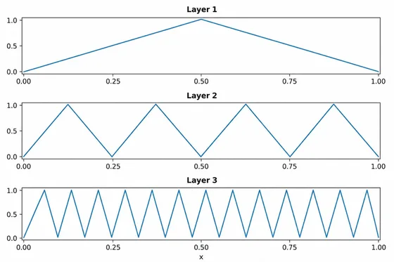
Figure 6. Repeated composition of the triangle wave. Each composition doubles the number of linear pieces, which is the source of the exponential growth in the depth-separation example.

Depth separation shows that the advantage of depth lies mainly in representational efficiency. A shallow network can still represent the same function. Depth separation changes the network size required to do so.

It is important to note that depth separation usually constructs worst-case functions. Whether functions in natural data really require this exponential width is a different question. That question leads to the hierarchical representation hypothesis and scaling laws.

Hierarchical Representation Hypothesis

Consider a photograph of a toucan. Humans classify images hierarchically. They first detect edges, curves, and textures, then combine them into eyes, a giant beak, feathers, claws, and a branch, and finally arrive at the concept “bird”. This process from pixels to parts to the whole object is hierarchical representation.

The hierarchical representation hypothesis argues that part of the effectiveness of deep networks comes from matching this hierarchical structure. Low-level convolution filters detect simple features. Middle layers combine them into local parts. High layers combine parts into complete objects. More layers allow more complex compositions.

This hypothesis is intuitively powerful, and it remains a hypothesis. It explains why depth may be useful. It does not provide a precise theorem that can be tested directly.

Figure 7. A toucan (Ramphastos toco). From pixels to features to parts to the whole object, natural images have a clear hierarchical structure.

Scaling Laws

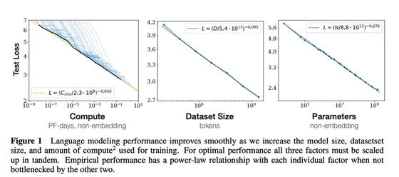
If depth separation emphasises representational efficiency, scaling laws focus on the empirical relationship between model scale and performance. Kaplan et al. (2020) found that the test loss of language models decreases as a power law when compute, data, and parameters increase.

L(C)=\left(\frac{C_{\min}}{2.3\times10^8}\right)^{-0.050},

L(D)=\left(\frac{D}{5.4\times10^{13}}\right)^{-0.095},

L(N)=\left(\frac{N}{8.8\times10^{13}}\right)^{-0.076}.

Here $C$ is compute, $C_{\min}$ is the minimum compute used for normalisation, $D$ is the number of training tokens, and $N$ is the number of non-embedding parameters.

These curves are approximately straight lines on a log-log plot, which means that loss follows a power law as scale increases. The paper also notes that, within reasonable limits, performance depends very weakly on other architectural hyperparameters such as depth versus width. Scale itself has a stronger effect.

Scaling laws and the UAT address different levels of the problem. The UAT says that a network has the capacity to represent a function. Scaling laws describe how loss changes with scale during actual training. One is an existence theorem, and the other is an empirical regularity.

Figure 8. Test loss of language models as a function of compute, dataset size, and parameters. The three curves are approximately straight on a log-log plot, showing power-law behaviour.

Hierarchical Composition in Natural Language

Natural language also exhibits hierarchical composition. Consider the following sentence.

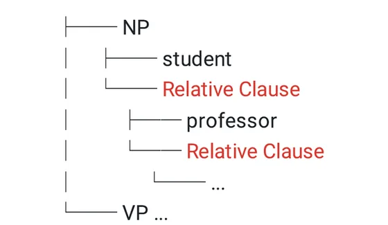
The student (who the professor (that I met yesterday) recommended) finally graduated.

The sentence contains nested relative clauses. The main clause is “the student finally graduated”. One relative clause modifies the student, and another relative clause modifies the professor.

Linguistics represents this structure with a syntax tree. Figure 9 shows a simplified example. NP splits into student and a Relative Clause, and the Relative Clause splits into professor and another Relative Clause. Each level combines smaller constituents.

The key observation is that natural language is hierarchical, and its hierarchy has a bounded depth. Everyday sentences have bounded nesting depth. Beyond a certain depth, sentences become difficult to understand. This observation matters for the discussion that follows.

Figure 9. A syntax tree for natural language. Sentences are built by combining phrases and clauses hierarchically, but the actual depth of nesting is usually limited.

Reconciling Two Perspectives

Depth separation and scaling laws seem to send different signals. Depth separation says that some functions need exponentially many neurons in a shallow network, so depth matters. Scaling laws say that, within reasonable limits, Transformer performance is relatively insensitive to the depth-width trade-off, and scale matters more.

One possible interpretation is that natural language does have hierarchical composition, but its compositional complexity is far below the worst-case theoretical constructions. The functions constructed in depth separation require exponentially many oscillations, while the actual nesting depth in natural language is usually limited.

Another interpretation is that Transformers may already operate beyond a critical depth. Beyond that depth, additional layers bring diminishing returns, and increasing width or data brings more benefit. GPT-3 (175B) contains 96 layers of Transformer decoder blocks, which is already a substantial depth.

Both are interpretations, and neither has been proven as a theoretical result. They remind us that there can be a large gap between worst-case theory and the data distributions we actually encounter.

Further Thoughts

Two questions remain open.

First, if Transformers already operate beyond a critical depth, why do increasingly large models continue to generalise well as they grow? Classical statistical learning theory often warns that excessive model capacity leads to overfitting, but the behaviour of large models does not fully match this intuition.

Second, scaling laws are currently empirical observations. Why does loss follow a power law? What determines the exponent? Is there a deeper theoretical explanation? These questions remain open.

Deep learning theory extends beyond the Universal Approximation Theorem. The theorem tells us what networks can represent. Modern deep learning is more concerned with how to represent functions efficiently, train them successfully, and generalise reliably.

Summary

The Universal Approximation Theorem shows that a single hidden layer is already capable of approximating any continuous function. This result answers a question about representational capacity. It does not address training algorithms, optimisation difficulty, or generalisation.

The constructive proof gives an intuitive path. A sigmoid can approximate a step function. Two step functions can form a local bump. Many bumps can form a continuous function. The one-dimensional construction extends to higher dimensions. Each step corresponds to a group of hidden neurons and a set of adjustable parameters.

Depth separation further shows that depth can greatly improve representational efficiency. Shallow networks still have the same representational capacity, but they may require far more neurons. Some functions with hierarchical composition require exponentially many neurons in a shallow network and only linearly many in a deep network.

The hierarchical representation hypothesis and scaling laws add two more perspectives. The first explains why depth may match the structure of natural data. The second describes the empirical relationship between scale and performance. Both remind us that the UAT is only a starting point.

In one sentence, the Universal Approximation Theorem tells us what neural networks can represent. Modern deep learning studies how to represent those functions efficiently, learn them successfully, and generalise well to unseen data.

References

Cybenko, G. (1989). Approximation by superpositions of a sigmoidal function. Mathematics of Control, Signals and Systems, 2(4), 303–314.
Hornik, K., Stinchcombe, M., & White, H. (1989). Multilayer feedforward networks are universal approximators. Neural Networks, 2(5), 359–366.
Nielsen, M. (2019). Neural Networks and Deep Learning. Chapters 4–5. http://neuralnetworksanddeeplearning.com/
Telgarsky, M. (2016). Benefits of Depth in Neural Networks. Proceedings of the 29th Conference on Learning Theory (COLT).
Kaplan, J., et al. (2020). Scaling Laws for Neural Language Models. arXiv:2001.08361.

This article is a written version of a presentation. The original slides are available as a PDF, 3.3 MB.

Figures 1–5 are adapted from Michael Nielsen's Neural Networks and Deep Learning, Chapter 4. Figure 6 is based on Telgarsky (2016), and Figure 8 is based on Kaplan et al. (2020). The toucan photograph in Figure 7 is from public image material and is used for teaching purposes only.